


A counterfactual is the outcome that would have occurred if a specific action had not been taken, or had been taken differently. In marketing measurement, it is the sales a brand would have made without a campaign, channel or budget change. The incremental effect is the difference between actual sales and this unobserved counterfactual.
Why the counterfactual cannot be observed
Every causal claim compares two states of the world. Each unit, such as a customer, a region or a week of sales, has one potential outcome with the treatment and another without it. The idea goes back to Neyman's work on agricultural field experiments (Neyman, 1923/1990) and was extended to observational studies by Rubin (1974). Only one of the two outcomes is ever observed. Once a campaign has run in a region, the sales that region would have had without the campaign cannot be measured. Holland (1986) called this the fundamental problem of causal inference.
Every method in causal inference is therefore a way of estimating a missing number, and an incrementality estimate is only as credible as the counterfactual behind it.
Formula and worked example
Incremental effect = Actual outcome − Counterfactual outcome
Incremental ROAS (iROAS) = (Actual revenue − Counterfactual revenue) / Ad spend
The counterfactual depends on the question. For a campaign launch, it is sales without the campaign. For a go-dark test, where advertising is paused, it is sales had advertising continued, so the effect shows up as lost sales. For a budget increase, it is sales at the previous budget.
Suppose a retailer runs a four-week online video campaign in one region and spends EUR 20 000. The region sold EUR 500 000 in the four weeks before the campaign and EUR 600 000 during it. Over the same weeks, comparable regions without the campaign grew by 14% because of seasonal demand. The table compares two counterfactuals for the same data:
| Metric | Before-after comparison | Control-based counterfactual |
| Actual sales during the campaign | EUR 600 000 | EUR 600 000 |
| Counterfactual sales | EUR 500 000 (pre-period sales) | EUR 570 000 (500 000 × 1.14) |
| Incremental sales | EUR 100 000 | EUR 30 000 |
| iROAS (incremental sales / EUR 20 000) | 5.0 | 1.5 |
With the same data and spend, the before-after comparison credits the campaign with seasonal growth that would have happened anyway. The numbers are illustrative.
How counterfactuals are estimated
Methods differ in where the counterfactual comes from and what makes it valid:
| Method | Source of the counterfactual | Key assumption |
| Randomized holdout (conversion lift study) | Randomly selected users who are not shown the ads | Randomization worked and the control group was not exposed |
| Geo test with control regions | Sales in untreated regions | Test and control regions would have moved together; no spillover |
| Synthetic control | Weighted combination of untreated regions that matches the pre-period | The pre-period fit carries over into the test period |
| Bayesian structural time series | Forecast of the test series, with control series as predictors | The relationship between test and control series is stable |
| Marketing mix model | Model prediction with a channel's spend set to zero or changed | The model captures confounders, carryover and saturation correctly |
Randomization gives the most reliable counterfactual, because chance rather than ad targeting decides who sees the ads, so a random holdout group shows what the exposed group would have done without them. When users cannot be randomized, for example for TV or offline sales, regions become the unit. The synthetic control method builds the counterfactual for a treated region as a weighted average of untreated regions (Abadie, Diamond & Hainmueller, 2010), and Bayesian structural time-series models forecast it from control series and return a posterior distribution of the effect (Brodersen et al., 2015).
Comparisons that look like counterfactuals often are not. Users who were exposed to an ad and users who were not are different people, because targeting selects users who are more likely to buy. Gordon et al. (2019) compared observational methods with 15 randomized advertising experiments at Facebook and found that the observational methods often failed to reproduce the experimental results, even after conditioning on extensive demographic and behavioral data.
Counterfactuals in incrementality experiments
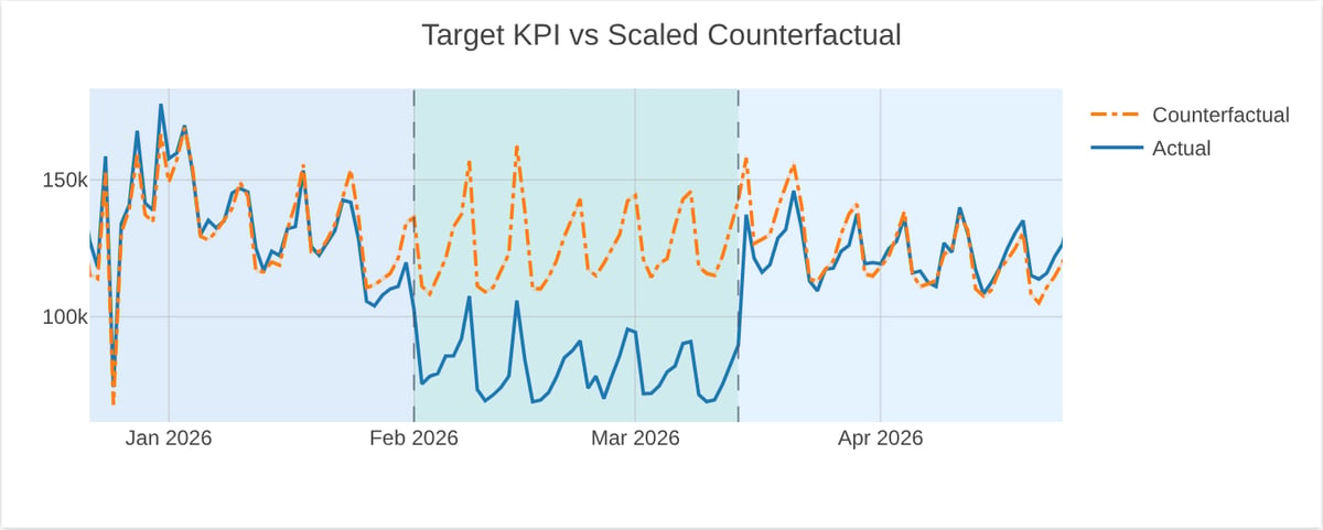
The chart below is from a go-dark geo lift test in the Sellforte demo (demo data), in which Meta and Google advertising was paused in one market for six weeks. The dashed line is the counterfactual, a weighted combination of untreated markets showing the sales the market would have made had advertising continued. The gap during the test period (shaded) is the estimated effect of pausing.
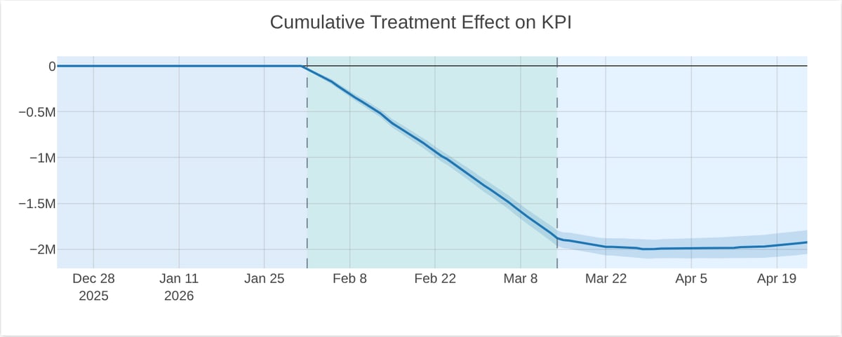
Summing the daily gaps gives the cumulative effect, shown below for the same demo test. The line keeps falling for a while after advertising resumes, a sign of carryover, or adstock. In a go-dark test, the spend in the iROAS calculation is also counterfactual: the spend that was withheld.
Because a counterfactual is never observed, its quality has to be checked indirectly:
- Pre-period fit. Before the test, the counterfactual should track actual sales closely; a poor fit makes the test-period estimate unreliable.
- Placebo tests. Running the same analysis at a date or in a market where nothing changed should find no effect (Abadie, Diamond & Hainmueller, 2010).
- Uncertainty. The counterfactual is an estimate with an interval, and its uncertainty carries over to iROAS.
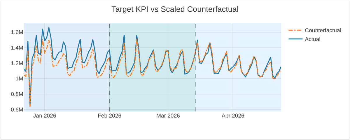
The last chart is a placebo check from the same demo (demo data), run on markets where nothing changed. During the placebo window (shaded), the counterfactual and actual sales move together, and the analysis finds no reliable effect, as it should.
Counterfactuals in marketing mix modeling
A marketing mix model does not observe a counterfactual either; it computes one. A channel's contribution is the difference between the model's predicted sales with actual spend and its predicted sales in a scenario where that channel's spend is set to zero, with everything else held as it was. Google's open-source MMM Meridian, for example, compares the expected outcome under historical media with a counterfactual in which a channel's media is set to zero, and divides this incremental outcome by spend to get the metric it calls ROI (Google, n.d.). Removing all media and price promotions at once gives the model's estimate of base sales.
The counterfactual should match the decision. Total contribution and iROAS show whether a channel has paid back so far, while budget decisions need a small change in spend from the current level. The change in predicted revenue per unit of extra spend is the marginal iROAS, which Meridian calls mROI.
Model-based counterfactuals have weak points. If a channel has always been on, a zero-spend scenario lies outside the observed data and depends on the model's functional form and priors. If the model omits a driver such as promotions, the counterfactual absorbs its effect. Experiment results are therefore used to calibrate MMM and anchor its counterfactuals to measured lift; Sellforte, for instance, calibrates its MMM with conversion lift studies.
Common mistakes
- Using the pre-period as the counterfactual. This ignores seasonality, trends and other changes, as in the example above.
- Comparing exposed and unexposed users. These groups differ in purchase intent, so the comparison overstates the effect.
- Treating attributed conversions as incremental. Attribution assigns credit to touchpoints in a customer journey; it does not estimate what would have happened without them.
- A contaminated control group. National TV that reaches control regions, or control users who see the same message elsewhere, pulls the counterfactual toward the actual outcome and hides the effect.
Key takeaways
- A counterfactual is what would have happened without the action. It is never observed and must be estimated.
- Incremental sales and iROAS are only as reliable as the counterfactual behind them.
- Randomized control groups give the most reliable counterfactuals; geo methods and MMM rely on assumptions that pre-period fit, placebo tests and calibration help to check.
- Choose the counterfactual to match the decision: zero spend for total contribution, a small spend change for marginal iROAS.
Related terms
- Incrementality
- Causal inference
- Causality
- Holdout group
- Conversion lift study
- Geo lift test
- Synthetic control method
- Base sales
Further reading on Sellforte
- What is incrementality testing?
- What is causal marketing mix modeling?
- Why can two analyses of the same holdout test produce different lift?
- MMM calibration explained
References
- Abadie, A., Diamond, A., & Hainmueller, J. (2010). Synthetic control methods for comparative case studies: Estimating the effect of California's tobacco control program. Journal of the American Statistical Association, 105(490), 493–505. https://doi.org/10.1198/jasa.2009.ap08746
- Brodersen, K. H., Gallusser, F., Koehler, J., Remy, N., & Scott, S. L. (2015). Inferring causal impact using Bayesian structural time-series models. The Annals of Applied Statistics, 9(1), 247–274. https://doi.org/10.1214/14-AOAS788
- Google. (n.d.). Incremental outcome, ROI, mROI & response curves. Meridian documentation. Retrieved November 16, 2026, from https://developers.google.com/meridian/docs/post-modeling/roi-mroi-response-curves
- Gordon, B. R., Zettelmeyer, F., Bhargava, N., & Chapsky, D. (2019). A comparison of approaches to advertising measurement: Evidence from big field experiments at Facebook. Marketing Science, 38(2), 193–225. https://doi.org/10.1287/mksc.2018.1135
- Holland, P. W. (1986). Statistics and causal inference. Journal of the American Statistical Association, 81(396), 945–960. https://doi.org/10.1080/01621459.1986.10478354
- Neyman, J. (1990). On the application of probability theory to agricultural experiments. Essay on principles. Section 9 (D. M. Dabrowska & T. P. Speed, Trans.). Statistical Science, 5(4), 465–472. https://doi.org/10.1214/ss/1177012031 (Original work published 1923)
- Rubin, D. B. (1974). Estimating causal effects of treatments in randomized and nonrandomized studies. Journal of Educational Psychology, 66(5), 688–701. https://doi.org/10.1037/h0037350
Authors

Dr. Paavo Niskala is a Principal Engineer at Sellforte. With PhD in the field of computational plasma physics, he has over 10 years of experience in designing and building complex data-intensive systems. Paavo has especially focused on using data science in critical business applications, such as Marketing Mix Modeling, which helps businesses make better marketing decisions. Follow Paavo in LinkedIn.


