


The synthetic control method is a causal inference technique that estimates the effect of an intervention on one unit, such as a region, by building a weighted combination of untreated units whose pre-intervention history closely matches the treated unit. The gap between the treated unit and this "synthetic control" after the intervention is the estimated effect.
Origins of the method
The method was introduced by Abadie & Gardeazabal (2003), who estimated the economic cost of terrorism in the Basque Country by comparing its GDP with a weighted combination of other Spanish regions. Abadie, Diamond & Hainmueller (2010) formalized the estimator and its inference in a study of California's 1988 tobacco control program (Proposition 99). They found that by 2000, annual per capita cigarette sales in California were about 26 packs lower than in its synthetic counterpart. Abadie (2021) later reviewed when the method gives reliable estimates, what data it requires and where it can fail.
The method addresses a common problem in causal inference: only one or a few units receive the treatment, and no single untreated unit is a good comparison. Instead of choosing one comparison unit by hand, the method lets the data choose a combination.
How the synthetic control method works
Suppose one region (the treated unit) receives a campaign, and J other regions (the donor pool) do not. The method proceeds in four steps:
- Collect a pre-period. Gather the outcome, for example weekly sales, for all regions over a period before the intervention. Predictors such as store count or population can be added.
- Find donor weights. Choose non-negative weights w1…wJ that sum to one, so that the weighted average of the donors tracks the treated region as closely as possible in the pre-period.
- Build the counterfactual. Apply the same weights to the donors' outcomes in the post-period. The result is the synthetic control: an estimate of what the treated region would have done without the intervention.
- Estimate the effect. The effect in each post-period week is the actual outcome minus the synthetic control outcome.
Because the weights are non-negative and sum to one, the synthetic control is an interpolation of real units, not an extrapolation. The weights are also usually sparse, so only a few donors get a non-zero weight, which makes the comparison transparent. A good pre-period fit is the main diagnostic: if the synthetic control cannot reproduce the treated unit's history, its post-period estimate is not credible.
Example
A retailer runs a four-week TV campaign in one of 20 regions. The method finds that a combination of three untreated regions (weights 0.45, 0.30 and 0.25) tracked the test region's weekly sales closely over the previous year. During the campaign, the test region sells EUR 108 000 per week, and the synthetic control predicts EUR 100 000. The estimated lift is EUR 8 000 per week, or EUR 32 000 over four weeks. With a media cost of EUR 16 000, the incremental ROAS (iROAS) is 2.0. The numbers are illustrative.
Synthetic control in marketing geo experiments
Geo experiments measure advertising effects by changing spend in some geographic areas and not in others. Vaver & Koehler (2011) describe the randomized version, where non-overlapping regions are randomly assigned to treatment and control. Randomization works well when there are many comparable regions. Many brands, however, operate in markets with a small number of regions, or need to test in a specific region for business reasons. A simple comparison between test and control regions is then sensitive to differences in size, seasonality and local trends.
The synthetic control method handles this situation well: it needs only one or a few treated regions and builds the comparison from the rest. It also fits a common marketing setup, where an advertiser turns a channel on or off in selected regions and measures the effect on total sales, including offline and untracked sales. Sellforte's geo tests follow this logic, and the resulting iROAS estimates can be used to calibrate a marketing mix model.
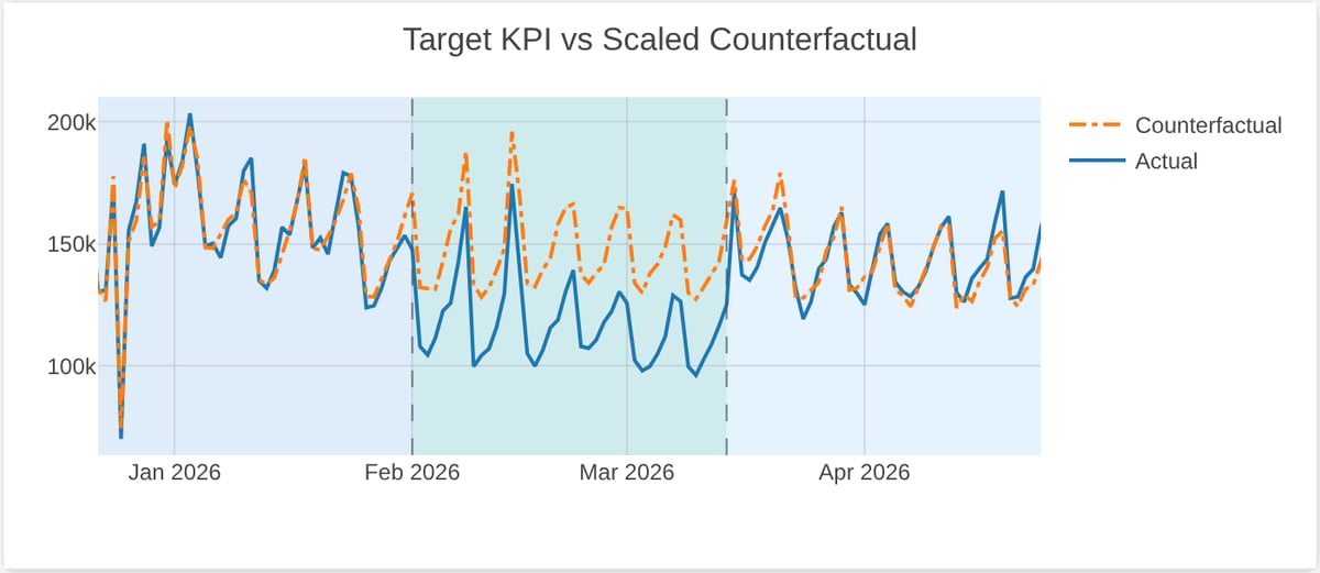
The chart below shows a synthetic control in practice, from a go-dark GeoLift test in the Sellforte demo (demo data). Before the test the counterfactual, a weighted combination of untreated markets, tracks actual sales closely; during the test period (shaded) the gap between the two lines is the estimated effect of pausing advertising.
Assumptions
The estimate is only as good as its assumptions. The most important ones, discussed in Abadie (2021), are:
- No spillover. The campaign must not affect donor regions. National TV, cross-region shoppers or online ads that leak across borders violate this.
- No other shocks to the treated unit. A store opening, a local promotion or a competitor's action in the test region during the test would be attributed to the campaign.
- A good, long pre-period fit. The synthetic control should track the treated unit over a long pre-period, ideally across seasons. A short pre-period invites overfitting.
- A comparable donor pool. Donors should be driven by similar factors as the treated unit. Because the weights cannot extrapolate, a treated region that is much larger or smaller than every donor cannot be matched well.
- No anticipation. The outcome must not react before the intervention starts, for example because of pre-announced promotions.
These assumptions are causal claims that the data alone cannot fully verify. A causal diagram of the market helps to see which events could break them.
Inference: placebo tests
With one treated unit, standard errors from large-sample theory do not apply. Abadie, Diamond & Hainmueller (2010) proposed permutation-style placebo tests instead:
- In-space placebos. Each donor is treated as if it had received the intervention, and a synthetic control is fitted for it. If the gap for the real treated unit is unusually large compared with these placebo gaps, the effect is unlikely to be chance. Comparing the ratio of post-period to pre-period fit error (RMSPE) accounts for placebos that were poorly fitted in the first place. The rank of the treated unit among all units gives a permutation p-value.
- In-time placebos. The intervention date is moved back into the pre-period. A credible model should show no "effect" at a date when nothing happened.
With few donors, the smallest attainable p-value is coarse: with 9 donors and one treated unit, it is 1/10 = 0.10. Small geo tests therefore need long tests or larger expected effects to give conclusive results.
Relation to difference-in-differences and Bayesian structural time series
| Method | How the counterfactual is built | Key assumption |
| Difference-in-differences (DiD) | Control group average, with equal weights, plus the pre-period level difference | Parallel trends between treated and control groups |
| Synthetic control | Weighted donor combination chosen to fit the pre-period | The pre-period fit carries over to the post-period; no spillover |
| Bayesian structural time series (CausalImpact) | State-space model of the treated series, with control series as regressors | The relationship between treated and control series is stable and unaffected by the intervention |
DiD can be seen as a special case with equal weights. When the treated unit follows a different trend from the average control, DiD is biased, while the synthetic control method can still find a combination that tracks it. Brodersen et al. (2015) take a related approach in a fully Bayesian framework: a structural time-series model predicts the counterfactual from control series and returns a posterior distribution of the effect. Their CausalImpact R package is widely used for marketing interventions.
Key takeaways
- The synthetic control method estimates a counterfactual for a treated region as a weighted average of untreated regions, chosen to match the pre-period.
- It suits geo experiments with few regions or a non-random test region, as long as there are no spillovers and the pre-period fit is good.
- Inference relies on placebo tests, and the number of donors limits how small the p-value can be.
Related terms
- Geo lift test
- Causal inference
- Causality
- Incrementality
- Bayesian statistics
- Directed acyclic graph (DAG)
Further reading on Sellforte
- What is incrementality testing?
- How should geo-lift and conversion-lift studies be combined when calibrating MMM?
- When is a market or channel too small to justify an incrementality test?
References
- Abadie, A. (2021). Using synthetic controls: Feasibility, data requirements, and methodological aspects. Journal of Economic Literature, 59(2), 391–425. https://doi.org/10.1257/jel.20191450
- Abadie, A., Diamond, A., & Hainmueller, J. (2010). Synthetic control methods for comparative case studies: Estimating the effect of California's tobacco control program. Journal of the American Statistical Association, 105(490), 493–505. https://doi.org/10.1198/jasa.2009.ap08746
- Abadie, A., & Gardeazabal, J. (2003). The economic costs of conflict: A case study of the Basque Country. American Economic Review, 93(1), 113–132. https://doi.org/10.1257/000282803321455188
- Brodersen, K. H., Gallusser, F., Koehler, J., Remy, N., & Scott, S. L. (2015). Inferring causal impact using Bayesian structural time-series models. The Annals of Applied Statistics, 9(1), 247–274. https://doi.org/10.1214/14-AOAS788
- Vaver, J., & Koehler, J. (2011). Measuring ad effectiveness using geo experiments. Google Inc. https://research.google/pubs/measuring-ad-effectiveness-using-geo-experiments/
Authors

Dr. Paavo Niskala is a Principal Engineer at Sellforte. With PhD in the field of computational plasma physics, he has over 10 years of experience in designing and building complex data-intensive systems. Paavo has especially focused on using data science in critical business applications, such as Marketing Mix Modeling, which helps businesses make better marketing decisions. Follow Paavo in LinkedIn.


