

Incrementality Testing Use Case

To check whether a geo-test result is robust in Sellforte, find the completed analysis in Experiments, then compare it with defensible alternative analyses of the same experiment. Review how the result changes with pretreatment history, cooldown and control selection, while keeping the intervention and business question consistent.
This guide uses the Meta + Google go-dark experiment in the public Sellforte demo. The analyses and figures are simulated. We compare existing completed analyses; no new analysis is run in this walkthrough.
Before you start: You need the primary geo analysis, its experiment plan and any completed sensitivity analyses. Define the decision threshold before interpreting differences.
What you will produce: A robustness readout showing which conclusions are stable and which depend on analysis choices.
1. Find the primary analysis and its alternatives
Open Experiments and search for Meta + Google go-dark. The demo returns four analyses of the February 1–March 14, 2026 intervention: the primary four-market analysis, a 14-day cooldown version, a two-year pretreatment version and an open donor-pool version.
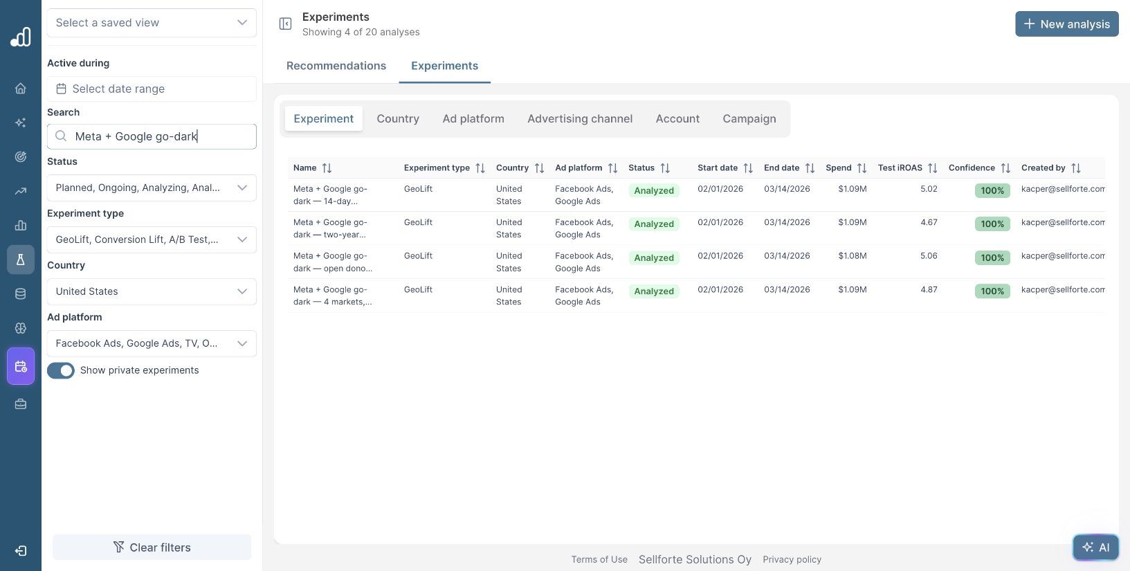
Open the primary result first. Record the country, tested media, dates and KPI, then confirm the test markets from the experiment setup. All four records concern a US go-dark experiment covering Facebook Ads and Google Ads. A combined-media test does not identify the separate return of each platform.
Use the analysis agreed for the main readout as the primary result. Choosing whichever version has the highest return after seeing the results would bias the conclusion.
2. Write down the primary estimate and uncertainty
The primary result shows iROAS of 4.87, with a displayed interval of 4.59–5.14. Incremental media spend is $1.09 million and incremental sales are $5.32 million. The model reports R² of 0.95, 364 observations and four predictors.
Record both the estimate and its interval. The question is whether reasonable analysis choices change the decision, not simply whether every point estimate is identical.
For a go-dark experiment, the treatment reduces media activity. The effect charts can therefore show negative spend and sales changes, while the headline return expresses the value of the withheld advertising. Keep that direction clear when writing the readout. See how to analyze the latest geo test for the initial results review.
3. Compare the cooldown and history choices
Return to the library and open the 14-day cooldown analysis. It reports iROAS of 5.02, with an interval of 4.68–5.36. A cooldown allows a defined period after treatment to capture effects that persist beyond the advertising change.
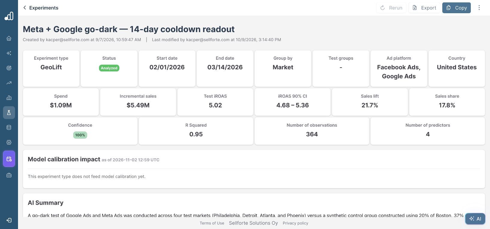
Use a cooldown supported by the expected response timing and experiment plan. Extending the window repeatedly until the result improves would make the comparison less trustworthy. Check for other activity during that period that could affect the outcome.
Next, open the two-year pretreatment analysis. It has 728 observations, compared with 364 in the primary analysis, and reports iROAS of 4.67, with an interval of 4.42–4.93.
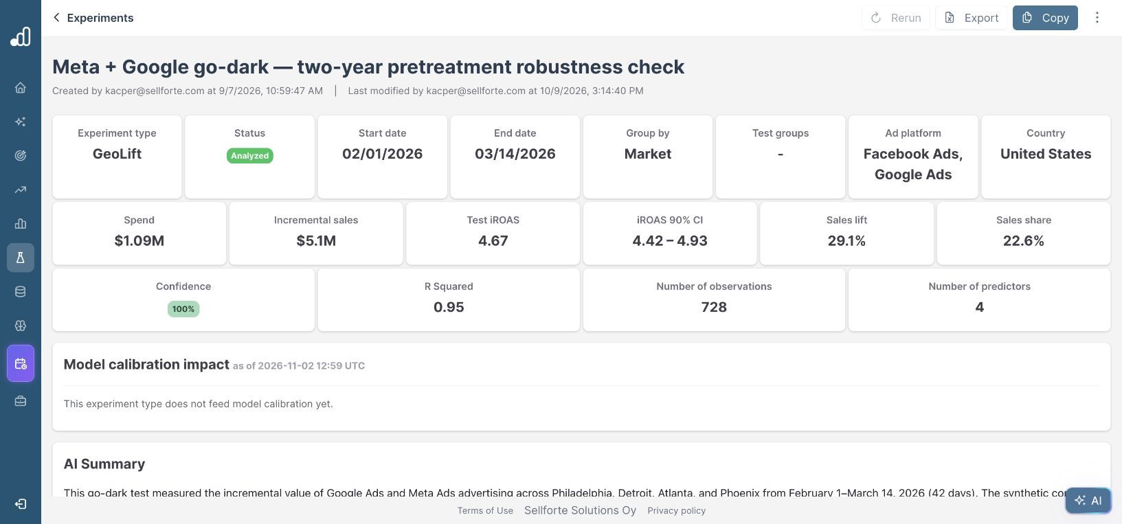
Longer history can provide more information about the relationship between test and control series. It can also introduce periods with different store coverage, measurement definitions or market conditions. Check that the historical data remain relevant rather than assuming that more observations always improve the analysis.
4. Inspect the control-pool alternative
Open the open donor-pool analysis. This version reports eight predictors rather than four, R² of 0.97 and iROAS of 5.06, with an interval of 4.87–5.26.
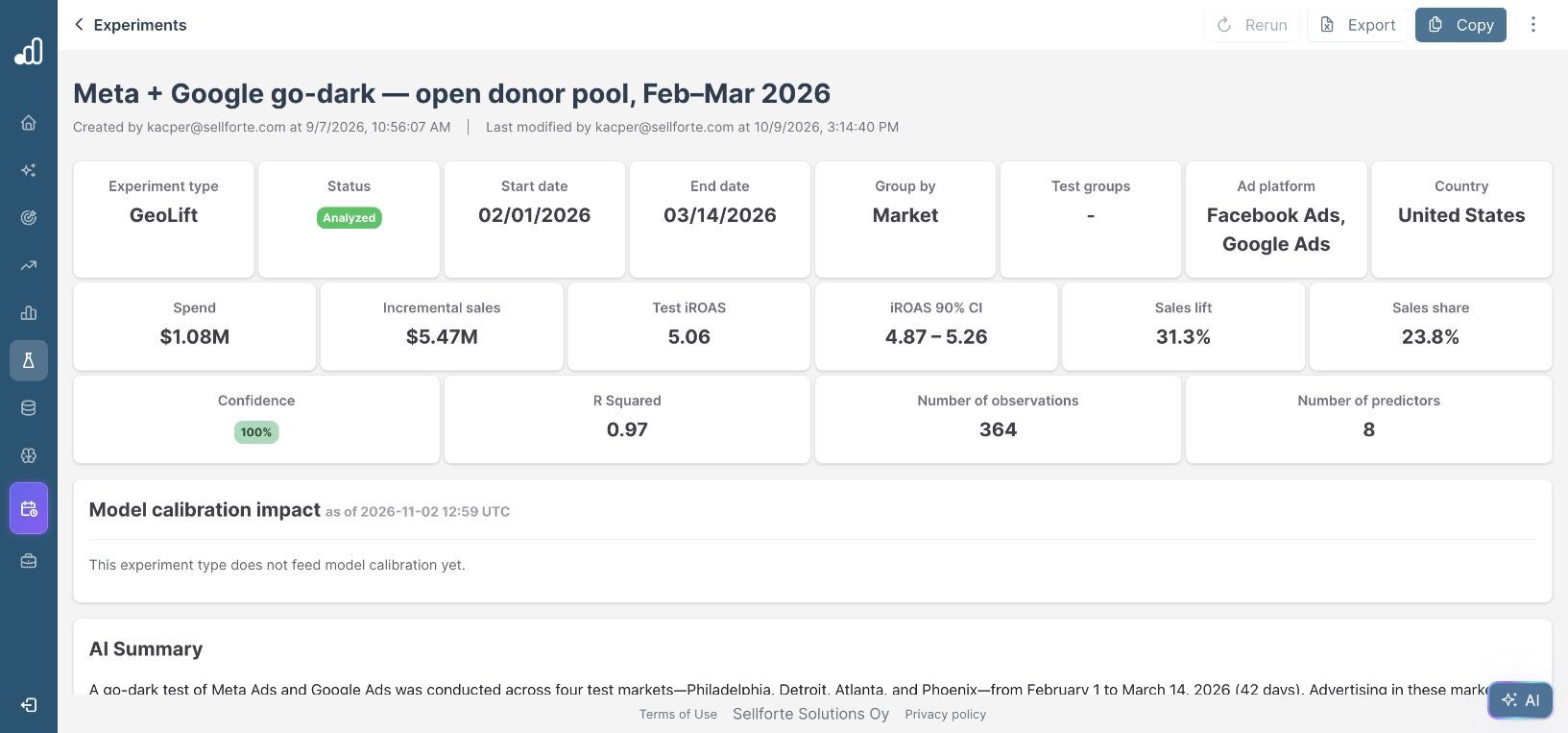
A donor pool is the set of candidate control series used to construct the counterfactual. Check that the controls were not exposed to the intervention or a closely related spillover. A better historical fit cannot make an affected control valid.
Review the actual-versus-counterfactual charts for pretest fit, unusual breaks and treatment timing. R² summarizes fit; it does not prove that the estimated effect is causal. Keep the control assignments and any exclusions in the analysis notes so the team can reproduce the comparison.
If you need to prepare these alternatives in your own workspace, the geo analysis setup guide shows the control and advanced-option fields. Change one assumption at a time where practical and name each version clearly.
5. Compare the results against the decision
| Analysis | Test iROAS | Displayed interval |
|---|---|---|
| Primary: four markets | 4.87 | 4.59–5.14 |
| 14-day cooldown | 5.02 | 4.68–5.36 |
| Two-year pretreatment | 4.67 | 4.42–4.93 |
| Open donor pool | 5.06 | 4.87–5.26 |
The point estimates range from 4.67 to 5.06, roughly 4% below or above the primary estimate. All displayed intervals remain positive. The broad conclusion that the tested media generated incremental sales is stable across these versions, subject to the experiment design and data being valid.
The business decision can still be sensitive to the threshold. For an illustrative required iROAS of 3.0, every displayed interval is above the threshold. For an illustrative threshold of 5.0, the evidence does not support the same clear conclusion across versions. Use your own KPI definition and economics to set that threshold.
These are four analyses of one experiment, not four independent replications. Do not average them into a new headline estimate or treat agreement as protection against an error shared by every version.
6. Save a readout that preserves the assumptions
“The primary geo analysis estimates iROAS at 4.87, with an interval of 4.59–5.14. Alternative cooldown, history and control-pool analyses produce point estimates of 4.67–5.06. The positive-return conclusion is stable, but a decision requiring iROAS above 5.0 remains uncertain. Retain the primary specification and document the alternatives.”
If the result changes direction or crosses an important decision threshold under a reasonable alternative, investigate the cause before using it to set budgets. The inconclusive test guide helps structure that follow-up.
Further Reading and Resources
Understand and configure the analysis
About the author

Lauri Potka is the Chief Operating Officer at Sellforte, with over 15 years of experience in Marketing Mix Modeling, marketing measurement and media spend optimization. Before joining Sellforte, he worked as a management consultant at the Boston Consulting Group, advising some of the world’s largest advertisers on marketing optimization. Follow Lauri on LinkedIn.


