MMM Use Case

To find room to scale, open Planning → Response curves in Sellforte and compare the expected return near each activity's current spend. Use the curve shape, observed spend range and marginal return together. A strong historical average return can coexist with little remaining headroom.
This walkthrough uses Meta Prospecting and Google Search Brand in New York in the public Sellforte demo. The displayed period is W27 August 2–W39 October 25, 2026. All screenshots and values use simulated demo data captured on November 15, 2026.
Before you start: You need access to response curves and a defined geography, outcome and planning horizon.
What you will produce: A shortlist of activities to investigate for increases or reductions, with the spend range and evidence limits recorded.
1. Narrow the comparison to a manageable scope
Open Response curves under Planning. Set the period, keep Country: US, and open Advertising channel. Select Deselect all, then choose Meta Prospecting and Google Search Brand. Use Back to return to the filters.
Open DMA, deselect the existing selection, and choose New York. Leave customer type, sales channel and product category at their displayed aggregate selections. The view states that it aggregates across those dimensions and splits by advertising channel and DMA. These are New York curves, not national channel totals.
2. Read the response curves at the spend markers
Stay on Compare with Response curve selected. The horizontal axis shows weekly spend and the vertical axis shows weekly Sales (MMM). Diamonds mark average weekly spend. The dotted segments are labeled Beyond observed spend.
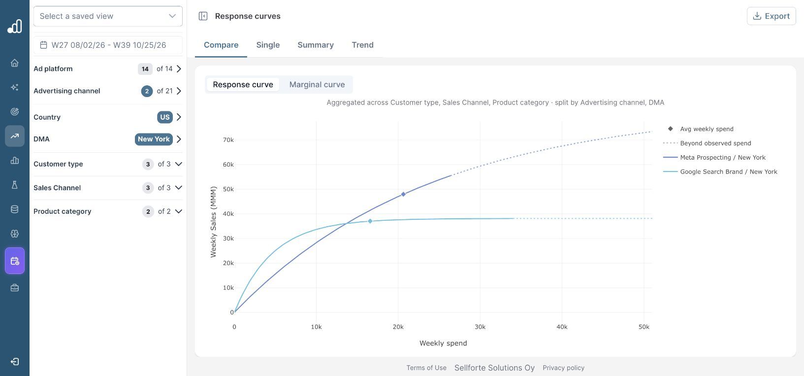
The branded-search curve is already quite flat around its marker. The prospecting curve is still rising more steeply around its marker. That is a reason to inspect the marginal-return figures, rather than judge the next increase from the height of either curve.
3. Confirm the numbers in Summary
Open Summary. The demo shows 13 weeks with spend for both rows.
| New York activity | Avg weekly spend | iROAS (period) | miROAS at avg spend |
|---|---|---|---|
| Meta Prospecting | $20.63k | 2.32 | 1.47 |
| Google Search Brand | $16.58k | 2.19 | 0.23 |
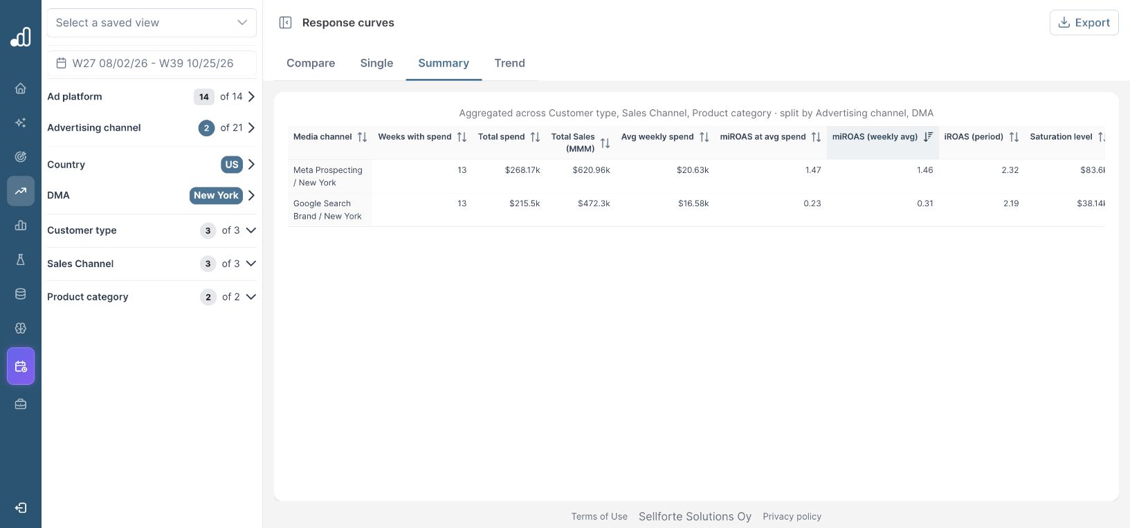
The period iROAS figures are relatively close, while the displayed marginal returns are very different. The same table also shows miROAS (weekly avg): 1.46 for prospecting and 0.31 for branded search. An average of weekly marginal returns need not equal the marginal return evaluated at average spend, because the response is nonlinear.
Do not read Saturation level as an approved spending cap. The table presents it alongside a response curve; the horizontal axis, observed-spend range and your business constraints are what you need to assess a proposed budget.
4. Inspect the marginal curves before proposing a change
Return to Compare and select Marginal curve. This plots marginal iROAS against weekly spend. It makes the declining return on additional investment easier to inspect.
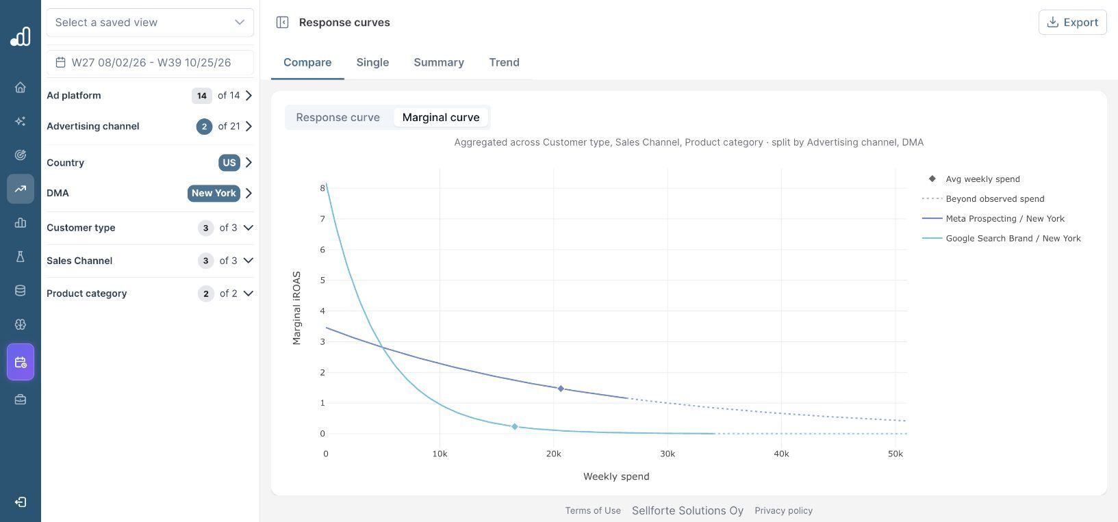
At the displayed average spend, prospecting is the stronger of these two candidates for an additional small investment. That does not automatically make an increase profitable. Compare the sales return with the business's contribution economics and account for uncertainty, operational limits and alternative uses of the budget.
For a finite change, compare modeled sales at both proposed spend levels. Avoid multiplying today's marginal return by an arbitrarily large budget increase. Recalculate after changing the allocation, particularly near or beyond the observed spend range. The miROAS guide explains the distinction in more detail.
5. Turn the comparison into a constrained scenario
In the selected New York demo scope, Meta Prospecting has 1.47 miROAS at average weekly spend, compared with 0.23 for Google Search Brand. Investigate a constrained reallocation toward prospecting, while checking the model's spend support, business requirements and the forecast for the complete plan.
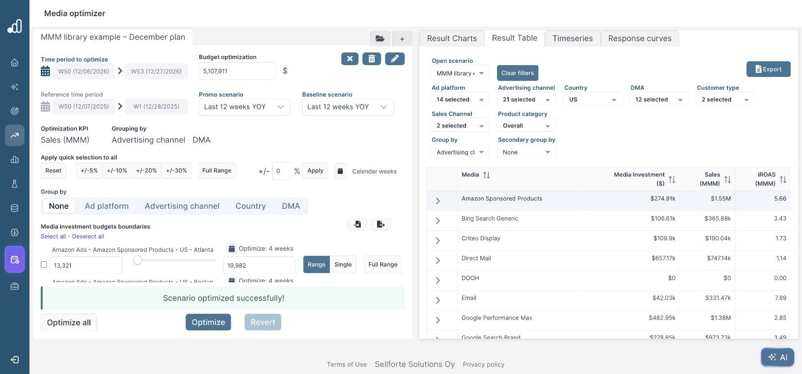
Take the candidate change into the Media optimizer and keep the same outcome and geography. A local curve comparison helps identify an opportunity; the full scenario checks whether that opportunity fits the rest of the budget and timing.
Further Reading and Resources
Understand the curves
Plan the next change
About the author

Lauri Potka is the Chief Operating Officer at Sellforte, with over 15 years of experience in Marketing Mix Modeling, marketing measurement and media spend optimization. Before joining Sellforte, he worked as a management consultant at the Boston Consulting Group, advising some of the world’s largest advertisers on marketing optimization. Follow Lauri on LinkedIn.
How to Compare MMM Results with Platform ROAS
How to See Which Channels Drive Incremental Sales