

To analyze an A/B test from your own files in Sellforte, open Experiments → New analysis → A/B Test. Upload the KPI history for your test and control groups, add media spend if you need iROAS, and set the treatment dates. The result shows the estimated incremental effect and its uncertainty.
This workflow fits an email holdout, catalog mailing or another controlled campaign whose data you want to bring into Sellforte. For example, you might want to answer: “Did our winback email generate additional sales?”
Before you start: Have access to Experiments, clearly defined test and control groups, KPI data from before and during the treatment, and the campaign dates. Prepare spend data if you want a return calculation.
What you will produce: An A/B test analysis and a short readout of the incremental outcome, return where available, and limitations.
The screenshots use the public Sellforte demo. Uploads and new analyses are disabled there. You can inspect the setup and follow the results section using its existing email winback test; all example figures are simulated.
1. Open a new A/B analysis
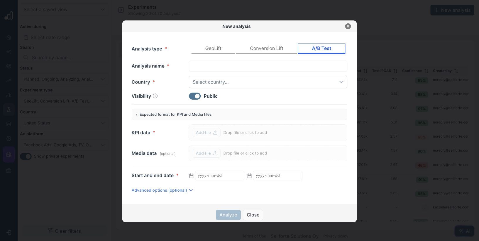
Choose Experiments in the left navigation, click New analysis, and select the A/B Test tab. Enter an Analysis name that identifies the activity, audience and period, such as “Email winback | Send vs holdout | April 2026”. Select the Country and review the Visibility setting for your workspace.
The form has a required KPI data upload and a separate, optional Media data upload. Use KPI data for the outcome you want to measure, such as daily sales value for the send and holdout groups.
2. Prepare the files using the built-in template
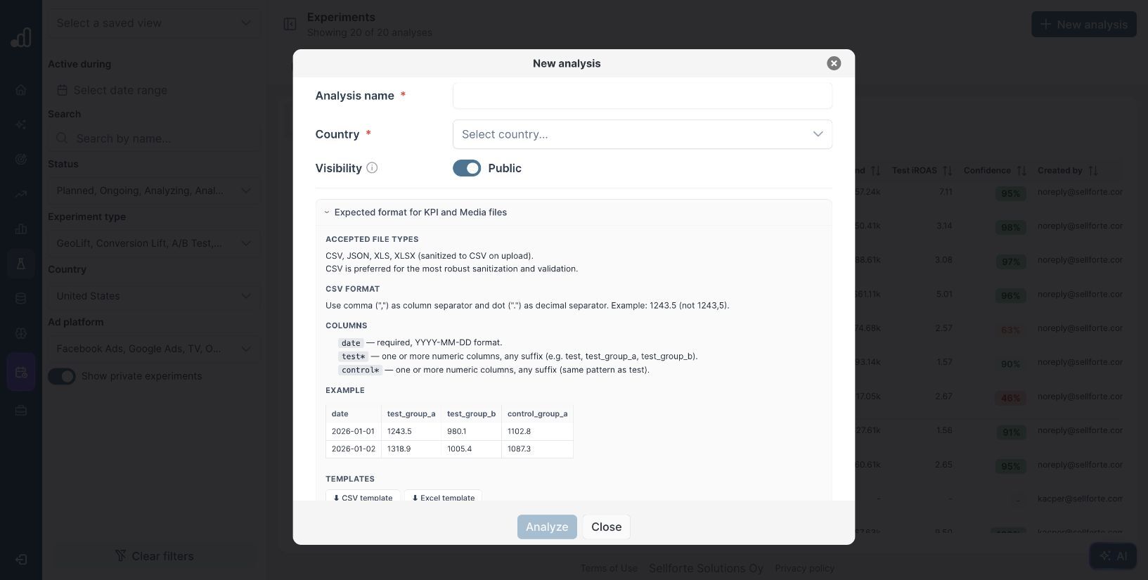
Expand Expected format for KPI and Media files. Download the CSV template or Excel template from this panel before arranging your data.
The form accepts CSV, JSON, XLS and XLSX. CSV is the recommended format. Use commas between columns and a dot for decimals: 1243.5. Follow the column structure shown in the panel:
| Column | What to put in it |
|---|---|
date | The observation date in YYYY-MM-DD format. |
test_send | A numeric KPI value for the group that received the campaign. |
control_holdout | The same KPI for a group held out from the campaign. |
The panel allows one or more numeric columns beginning with test and one or more beginning with control. Descriptive names such as test_send and control_holdout make the groups easier to recognize later.
Include history from before the campaign as well as the measurement period. Sellforte uses the earlier relationship between groups to estimate what the test group would have done without the campaign. A file containing only the campaign dates leaves out that comparison history.
Before uploading, check that the groups use the same KPI definition and units, the dates cover the intended analysis window, and the holdout was kept out of the treatment. Check missing or duplicated dates rather than silently treating missing observations as zero.
3. Upload the data and set the treatment dates
In your Sellforte account, use Add file under KPI data or drop the file into that area. Wait for validation and resolve any reported date or column-name errors.
Add the spend file under Media data (optional) if you want iROAS. It follows the same date-and-group structure, with spend values instead of the KPI. Without media data, the analysis can estimate the incremental KPI effect, but it will not calculate iROAS.
Set Start and end date to the treatment period. These dates describe when the campaign ran; the uploaded file should also contain the earlier history used to establish the baseline.
Open Advanced options (optional) if your analysis plan calls for either of these settings:
- Pretreatment start date: Choose the beginning of the historical comparison window. Leaving it empty uses the first available date in the data.
- Cooldown period (days): Extend measurement beyond the campaign end to capture delayed effects. Include data covering that additional period.
Confirm that the files, group definitions and dates match your experiment plan, then click Analyze. Once processing finishes, open the analyzed experiment from the library.
4. Check the scope before reading the result
For a worked example, open Email winback push: send vs holdout A/B, Apr 2026 in the demo. This is a separate, pre-existing example, not an analysis of the template rows.
The header identifies an A/B Test with status Analyzed, covering April 5 to May 2, 2026 in the United States. The test group is test_Winback_Send. Farther down, the Control groups table identifies control_Winback_Holdout.
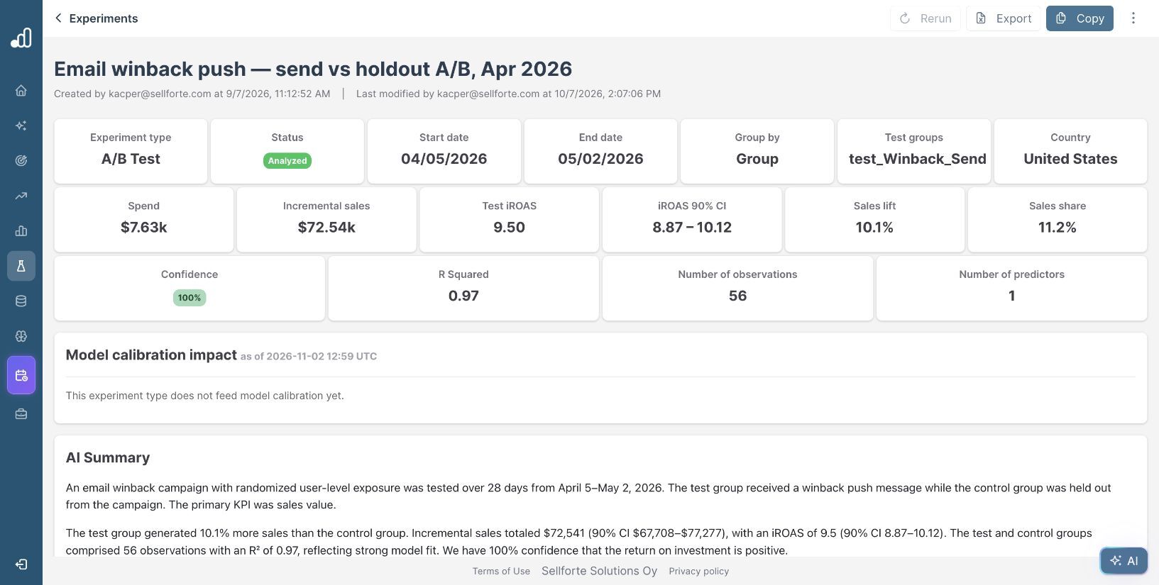
Read the main results together:
| Result | Demo value | How to use it |
|---|---|---|
| Incremental sales | $72.54k | The estimated sales added by the campaign. |
| Test iROAS | 9.50 | Incremental revenue per dollar of incremental investment. |
| iROAS 90% CI | 8.87 to 10.12 | The model’s credible range around the return estimate. |
| Sales lift | 10.1% | The estimated relative increase against the no-treatment baseline. |
| R Squared | 0.97 | A summary of historical fit; inspect the chart as well. |
The displayed Confidence is 100% in this demo. Treat it as a model-based result for this experiment. It does not guarantee that a different audience or a larger campaign will produce the same return.
5. Review the charts and write the readout
Scroll to Target KPI vs Scaled Counterfactual. Compare the actual and counterfactual lines before treatment, then examine their separation during the campaign. A close historical fit helps support the comparison; unusual events or treatment reaching the control group still need to be considered.
Next, read Cumulative Treatment Effect on KPI. It shows how the estimated effect accumulates over time. Check whether that timing makes sense for the campaign and whether effects continue after treatment ends.
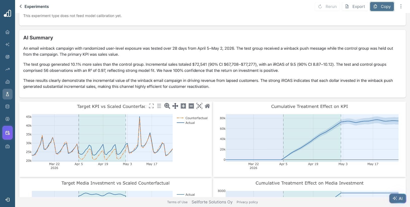
Use the AI Summary as a starting point, then check its claims against the setup, charts and uncertainty. A concise readout for this example could be:
The US email winback holdout test ran from April 5 to May 2, 2026. In the simulated demo, Sellforte estimates $72.54k in incremental sales, a 10.1% sales lift and 9.50 test iROAS, with a 90% credible interval of 8.87 to 10.12. The historical fit is strong at R² 0.97. Before repeating or expanding the campaign, compare the return with campaign costs and margins, and check how the next audience differs from the tested group.
Keep the experiment link with your readout so colleagues can inspect the same evidence. For a deeper explanation of the charts, continue with the guide to analyzing a completed geo test, which uses the same core counterfactual result views.
Further Reading and Resources
Set up and understand your analysis
Continue with incrementality testing
About the author

Lauri Potka is the Chief Operating Officer at Sellforte, with over 15 years of experience in Marketing Mix Modeling, marketing measurement and media spend optimization. Before joining Sellforte, he worked as a management consultant at the Boston Consulting Group, advising some of the world’s largest advertisers on marketing optimization. Follow Lauri on LinkedIn.

How to Find Previous Tests for a Channel or Market | Incrementality Testing Use Case

How to Decide What to Test Next | Incrementality Testing Use Case