


Difference-in-differences (DiD) is a causal inference method that estimates the effect of an intervention by comparing how an outcome changed over time in a treated group with how it changed in an untreated control group over the same period. In marketing, it estimates the incremental sales from a campaign or a spend change, for example in a geo test.
How difference-in-differences works
A before-and-after comparison mixes the effect of a campaign with everything else that changed at the same time, such as seasonality or promotions. A comparison between a test group and a control group mixes it with permanent differences between the groups, such as size. Difference-in-differences removes both: the change in the control group shows how the test group would have changed without the intervention, and what remains is the effect.
A classic application compared fast-food restaurants in New Jersey, where the minimum wage rose in April 1992, with restaurants in eastern Pennsylvania, where it did not, and found no indication that the increase reduced employment (Card & Krueger, 1994). In marketing, the treated group is usually a set of regions where media spend changes, and the control group a set of regions where it does not.
Formula
With one test group, one control group, one period before the intervention (pre) and one during it (post), the estimate is:
DiD = (Ytest, post − Ytest, pre) − (Ycontrol, post − Ycontrol, pre)
Here Y is the average outcome, such as weekly sales, in each group and period. With many regions and days, the same idea is usually estimated as a two-way fixed effects regression with a separate intercept for each region and each period (Angrist & Pischke, 2009). Dividing the incremental sales by the change in media spend gives the incremental ROAS (iROAS) of the tested media.
Worked example
A retailer adds EUR 10 000 per week of paid social spend in its test regions for six weeks, EUR 60 000 in total, and leaves the control regions unchanged:
| Group | Pre-period, weekly average | Test period, weekly average | Change |
| Test regions | EUR 400 000 | EUR 452 000 | +EUR 52 000 (+13.0%) |
| Control regions | EUR 600 000 | EUR 630 000 | +EUR 30 000 (+5.0%) |
| Difference (test − control) | EUR −200 000 | EUR −178 000 | +EUR 22 000 |
In levels, DiD = EUR 52 000 − EUR 30 000 = EUR 22 000 per week. But the control regions are 1.5 times larger, and their increase is 5.0%. If the test regions would also have grown 5.0%, their counterfactual is EUR 420 000, not EUR 430 000:
| Parallel trends assumption | Counterfactual test-region sales per week | Incremental sales per week | Incremental sales, 6 weeks | iROAS on EUR 60 000 |
| Same change in euros | EUR 430 000 | EUR 22 000 | EUR 132 000 | 2.2 |
| Same change in percent | EUR 420 000 | EUR 32 000 | EUR 192 000 | 3.2 |
Each version rests on a different parallel trends assumption. When groups differ in size, parallel trends in percent (a DiD on log sales) is often more plausible, because seasonal swings scale with market size. Choose the version before seeing the result, based on which fits the pre-period better. The numbers are illustrative.
The parallel trends assumption
DiD does not require the groups to have similar sales, only that without the intervention their outcomes would have changed by the same amount (Angrist & Pischke, 2009). This concerns the test period, when the counterfactual is unobserved, so it can never be fully verified. The usual evidence is the pre-period: groups that moved together for months before the test probably would have kept doing so. In marketing, the assumption tends to fail when:
- Seasonality differs. A ski region and a beach region peak in different months.
- Something else changes locally. A store opening or regional promotion during the test is credited to the media.
- Effects spill over. National media or shoppers crossing regional borders also reach the control group, biasing the estimate toward zero.
- Test regions were chosen for a reason. Regions picked for a heavy-up because they were growing would show that growth as lift.
Inference and common pitfalls
Bertrand, Duflo and Mullainathan (2004) assigned placebo "laws" at random to US states and found that conventional standard errors showed an effect significant at the 5% level in up to 45% of cases, because outcomes are correlated over time. Daily regional sales behave the same way, so treating every region-day as independent makes a geo test look far more precise than it is. Collapsing the data into one pre-period and one post-period worked well even with few states, the typical geo-test situation.
Staggered rollouts, where regions start at different times, cause a second problem. The standard two-way fixed effects estimate is then a weighted average of all two-group, two-period comparisons, including ones that use already-treated regions as controls, and it is biased when the effect changes over time (Goodman-Bacon, 2021), as advertising effects with adstock do. Roth et al. (2023) review newer estimators for these settings.
Difference-in-differences for incrementality testing
In a geo lift test, DiD is the most transparent way to build the counterfactual. It works best with many comparable regions and a clear change in spend. With few regions, or test regions that follow a different pattern from the average control region, an equally weighted control group is a poor match. The synthetic control method instead weights the control regions to reproduce the test regions' pre-period sales.
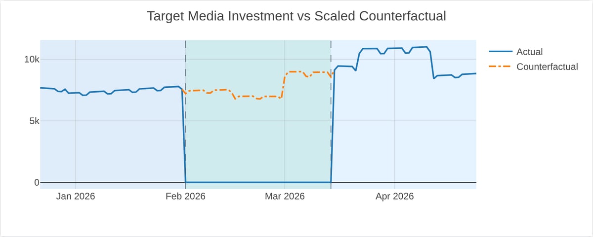
The charts below are from a single-market go-dark geo test in the Sellforte demo (demo data). First, the treatment: paid media in the test market was switched off for six weeks.
Second, sales in the same market. Before the test, actual sales and the counterfactual move together, the visual check behind parallel trends; the gap during the test is the estimated incremental sales.
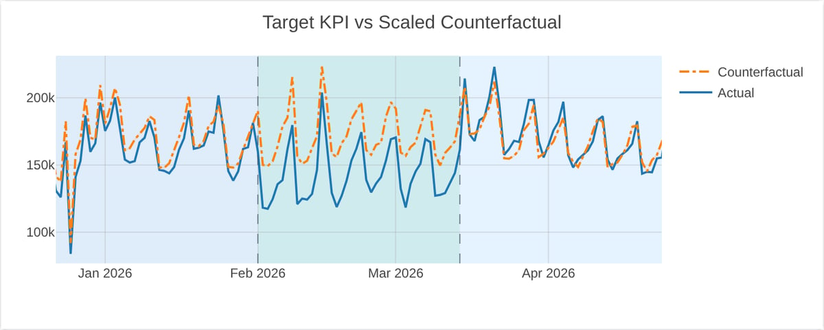
This counterfactual comes from a synthetic control that puts 63% of the weight on Minneapolis-St. Paul and 27% on Dallas-Fort Worth; a plain DiD would weight every control market equally.
Synthetic difference-in-differences combines the two: like synthetic control, it weights control units to match the treated units' pre-period trend; like DiD, it allows a constant level difference; and it also weights pre-period time points (Arkhangelsky et al., 2021). Bayesian structural time-series models generalize DiD to time series and show how the effect evolves (Brodersen et al., 2015). Sellforte's April 2026 Experiments Hub announcement describes its geo lift analysis as Bayesian synthetic control, with Bayesian synthetic DiD as the planned upgrade. If DiD and synthetic control disagree sharply, at least one assumption probably fails.
Difference-in-differences and marketing mix modeling
A marketing mix model estimates every channel's effect from spend variation over time and markets, controlling for seasonality, prices and promotions. A DiD estimate comes from one deliberate change in a few regions. The two complement each other:
- Calibration. A geo test's iROAS can serve as prior information to calibrate the marketing mix model, once matched to the same channel, KPI and period.
- Validation. If the model's iROAS falls well outside the test's interval, the model or the test design needs a closer look.
- Natural experiments. A TV flight in some regions only or a channel paused in one market can be analyzed with DiD, if the timing was not driven by local demand.
- Test design. The model's iROAS shows how large a spend change is needed for the effect to stand out from noise. Keeping comparable regions at normal spend preserves the comparison DiD needs, as the post on full blackouts versus partial holdouts explains.
Key takeaways
- DiD estimates an effect as the change in the test group minus the change in the control group.
- It relies on parallel trends, which pre-period data can support but never prove.
- Decide in advance whether trends should be parallel in euros or in percent; the choice can change the iROAS considerably.
- Standard errors that ignore correlation over time overstate precision.
- With few regions, synthetic control or synthetic DiD often fits better; test-based iROAS helps calibrate and validate MMM.
Related terms
- Synthetic control method
- Geo lift test
- Counterfactual
- Causal inference
- Minimum detectable effect (MDE)
- Holdout group
- Incrementality
- Adstock
Further reading on Sellforte
- Why can two analyses of the same holdout test produce different lift?
- Should we run a full marketing blackout or a partial holdout test?
- Introducing Sellforte Experiments Hub
- What is incrementality testing? A practical guide
References
- Angrist, J. D., & Pischke, J.-S. (2009). Mostly harmless econometrics: An empiricist's companion. Princeton University Press. https://doi.org/10.1515/9781400829828
- Arkhangelsky, D., Athey, S., Hirshberg, D. A., Imbens, G. W., & Wager, S. (2021). Synthetic difference-in-differences. American Economic Review, 111(12), 4088–4118. https://doi.org/10.1257/aer.20190159
- Bertrand, M., Duflo, E., & Mullainathan, S. (2004). How much should we trust differences-in-differences estimates? The Quarterly Journal of Economics, 119(1), 249–275. https://doi.org/10.1162/003355304772839588
- Brodersen, K. H., Gallusser, F., Koehler, J., Remy, N., & Scott, S. L. (2015). Inferring causal impact using Bayesian structural time-series models. The Annals of Applied Statistics, 9(1), 247–274. https://doi.org/10.1214/14-AOAS788
- Card, D., & Krueger, A. B. (1994). Minimum wages and employment: A case study of the fast-food industry in New Jersey and Pennsylvania. American Economic Review, 84(4), 772–793. https://www.jstor.org/stable/2118030
- Goodman-Bacon, A. (2021). Difference-in-differences with variation in treatment timing. Journal of Econometrics, 225(2), 254–277. https://doi.org/10.1016/j.jeconom.2021.03.014
- Roth, J., Sant'Anna, P. H. C., Bilinski, A., & Poe, J. (2023). What's trending in difference-in-differences? A synthesis of the recent econometrics literature. Journal of Econometrics, 235(2), 2218–2244. https://doi.org/10.1016/j.jeconom.2023.03.008
Authors

Dr. Paavo Niskala is a Principal Engineer at Sellforte. With PhD in the field of computational plasma physics, he has over 10 years of experience in designing and building complex data-intensive systems. Paavo has especially focused on using data science in critical business applications, such as Marketing Mix Modeling, which helps businesses make better marketing decisions. Follow Paavo in LinkedIn.


