
The Response Curves view shows how sales respond to media spend for every channel in your model. It sits under Media Optimizer and plots the same curves the optimizer uses when it builds budget scenarios and the recommendations shown on Home. The view exists so that planners can see, before running a scenario, where each channel still has room to grow, where it is saturating, and how its efficiency has changed over time.
Why this view exists
Response curves have historically lived in Custom Reports or in the admin area, where they were hard to compare across channels and markets. The Response Curves view brings them into one place. You pick a time range on the left, and the curves are seasonality adjusted for that range, so a high season week and a low season week become directly comparable. Selecting a single week shows the exact curve applied to that week.
Four tabs, four questions
The page has four tabs at the top. Each one is built to answer a different question, so start from the question you have.
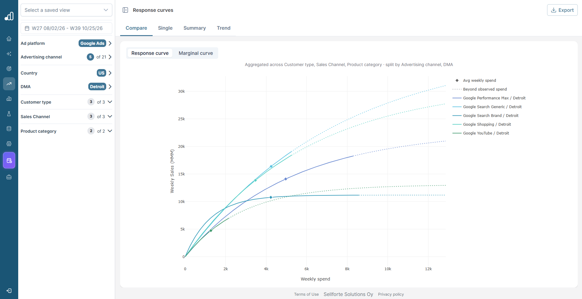
Compare: which channels still have headroom? Compare overlays several curves at once, split by the dimensions you choose in the filter panel. The caption above the chart states what the curves are aggregated across and what they are split by, so you always know what one line represents. With hundreds of curves split by channel, market, and campaign type, this is the practical planning tool: overlaying them turns a long list into a quick read of where extra spend still pays off. Compare shows the fitted curves and a diamond for the average weekly spend on each, but not the weekly data points.
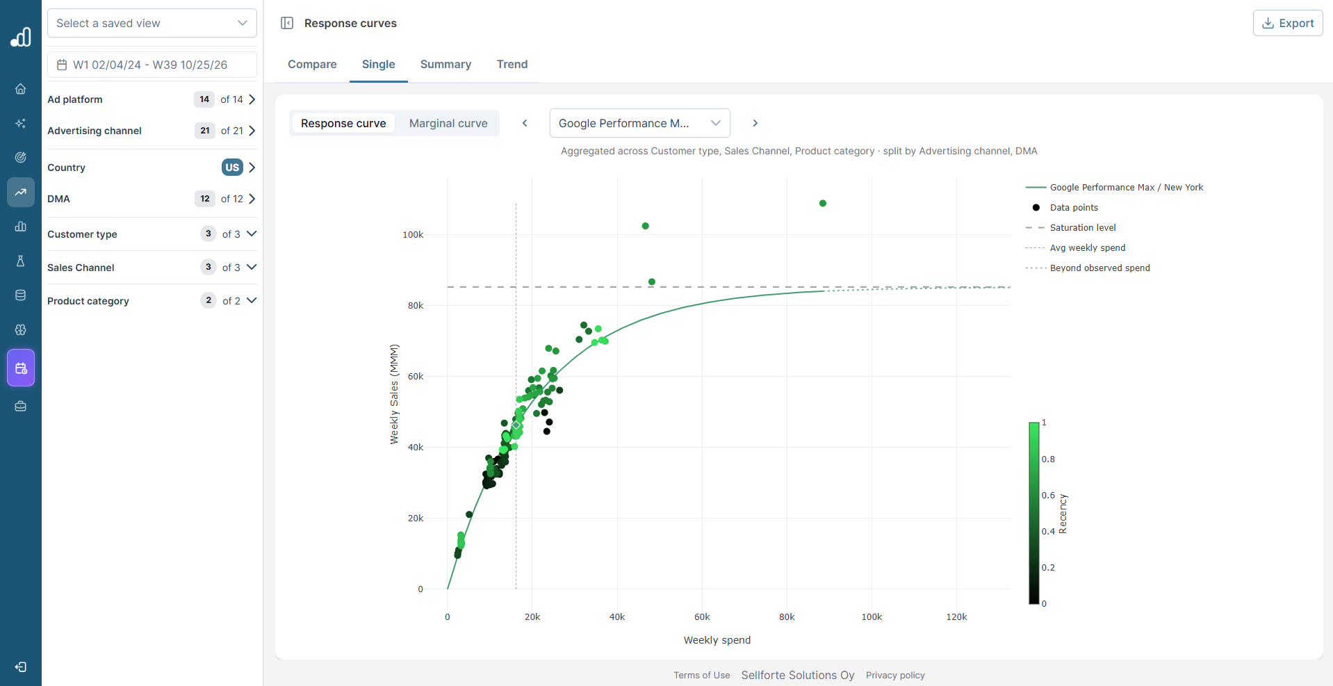
Single: what is behind this one curve? Single focuses on one curve and plots every weekly observation behind it. Use it when a Compare chart raises a question about a specific channel: are recent weeks above or below the fit, how many observations are there, and where do the high spend weeks sit.
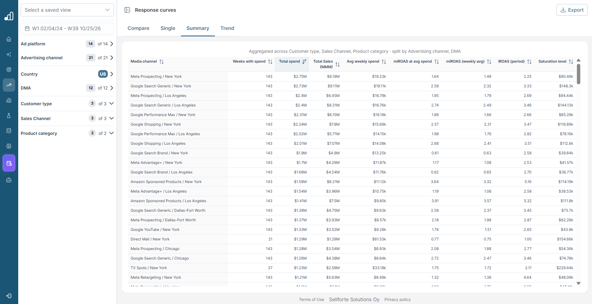
Summary: what are the numbers? Summary lists the selected curves in a table with weeks active, spend, incremental sales, average iROAS, and saturation level. Use it when you want to compare figures rather than shapes, or export them.
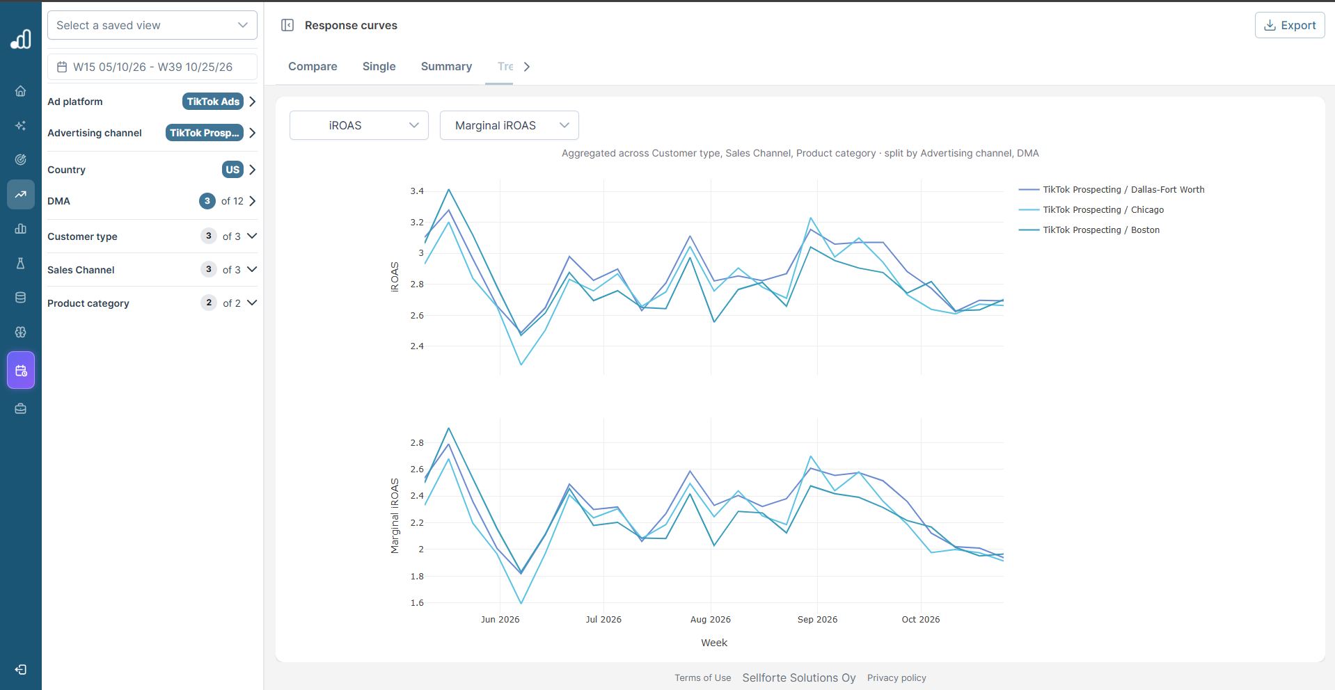
Trend: is efficiency stable, seasonal, or drifting? Trend shows how the selected metrics changed week by week. If iROAS falls while spend rose, the channel is simply moving up its own curve. If iROAS falls while spend stayed flat, the channel itself has become less effective, and that is a signal to investigate the channel rather than the plan.
Response curve or Marginal curve: two more questions
Inside Compare and Single, a second toggle switches between Response curve and Marginal curve. Both come from the same model, but each answers its own question.
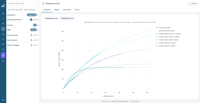
Response curve: how much, and how close to the ceiling? It plots weekly spend against weekly incremental sales. Where the diamond sits matters: on the steep part there is still room to grow, and on the flat part extra spend adds little. The gap between the current level and the saturation line is the headroom.
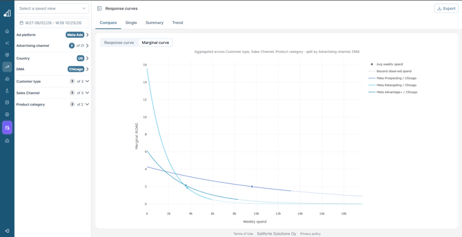
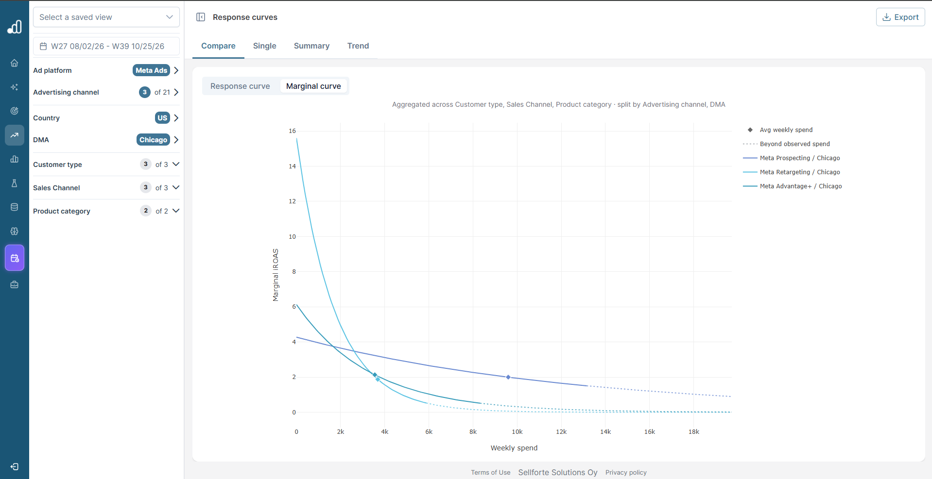
Marginal curve: where should the next euro go? It plots weekly spend against marginal iROAS. Two channels can have the same average iROAS but very different marginal iROAS, and moving budget from a low marginal iROAS channel to a high one increases total incremental sales. A marginal iROAS of 1 is break even in revenue terms only; the profit break even is higher and depends on your margin.
How to read a response curve
Each curve shows the model's best estimate of the relationship between spend and incremental sales. A steep start means the channel is still efficient at low spend. As the curve flattens, extra euros add less and the channel is saturating. Where the line is solid, the model is working within weekly spend levels it has seen in your data. Where the line turns dotted, it is extrapolating past the highest weekly spend ever observed, and that section is less certain and should be read as directional. The legend labels this section Beyond observed spend.
A diamond marks the average weekly spend in the selected period, so you can see at a glance where you currently sit on the curve. A grey saturation line marks the ceiling, which is the most weekly incremental sales the model believes the channel could ever drive, however much you spend.
In Single, every week of history is plotted as a dot. The sales value on each dot is the modeled incremental sales for that week's spend, with the model's carry over already applied, so a spend week still carries the effect it drove in the weeks that followed. The dots are seasonality adjusted against the base demand, so weeks across the year sit on a common baseline. A Black Friday week is a good example: a high spend week during high organic demand is adjusted back toward a normal week, so it does not dominate the fit.
Dots are colored by recency. Green dots are recent weeks and black dots are older ones, and the shades are spaced by date rather than by order. If recent dots sit below older ones, the same uplift now needs more spend and effectiveness has declined. If recent dots sit above the curve, the channel is saturating later than the model assumed.
How it fits the workflow
Response curves are the quantitative backbone of budget decisions in Sellforte. The Media Optimizer uses them to build scenarios, and Performance Recommendations use the marginal iROAS from these curves to suggest where to shift spend next week. Opening the Response Curves view directly is useful when you want to understand a recommendation, challenge a scenario, or brief a channel team on where the data says their channel is heading. A typical sequence is Compare to spot the channels that stand out, Single to dig into one of them, Summary for the numbers, and Trend when the question is about change over time.
Data requirements
A response curve needs enough weekly observations at a mix of spend levels to be reliable. Channels with little historical variation in spend produce a narrower band of observed data, and the curve is read with more caution outside that band. When a curve carries fewer observations than usual, lean on the solid portion and treat the dotted extension as directional. Curves are rebuilt daily from the latest model, so new observations show up on the next refresh.