Advertising response curves: What are they and why do you need them?

Advertising Response Curves (ARC) are one the most critical concepts to understand when optimizing media spend allocation across channels and campaigns. Advertising Response Curves represent a function in Marketing Mix Modeling (MMM) that describe the relationship between advertising spend and incremental sales driven by the channel or campaign.

This article discusses the intricacies of Response Curves, detailing their function, significance, and how they intersect with critical elements such as saturation points. We will also investigate the impact Response Curves have on Media Mix Optimization, specifically, the Return on Investment (ROI), and shed light on the various industry-standard types of curves. Lastly, we will deep dive into the process of building Response Curves.

What are Advertising Response Curves?

Advertising Response Curves represent a function that describes the relationship between the amount of money spent on advertising and incremental sales driven by marketing. While incremental sales is the most commonly use consumer response metric, it can theoretically also be replaced with other metrics, like brand awareness.

A Response Curve comprises two key elements: the level of advertising spend and the consumer response. Advertising spend typically appears on the x-axis, representing the amount of money spent on an advertising campaign, and the y-axis indicates the consumer response, portraying the reaction to the advertising campaign, usually in terms of sales or conversions.

In the example chart below, you can see Response Curves illustrated on the Sellforte platform. The chart shows Response Curves for various media channels, such as Google Search Generic, Google Search Brand, and so on. On the x-axis, we have media spend, and on the y-axis we have Incremental Sales that can be achieved during a week with the specified spend level.

Use-cases: How Can Marketers use Advertising Response Curves?

Use-case 1: Identify Level of Saturation

One of the main benefits of response curves is their ability to identify the level of saturation for each channel. As an example, let's analyse the image below, which represents a response curve for one individual channel.

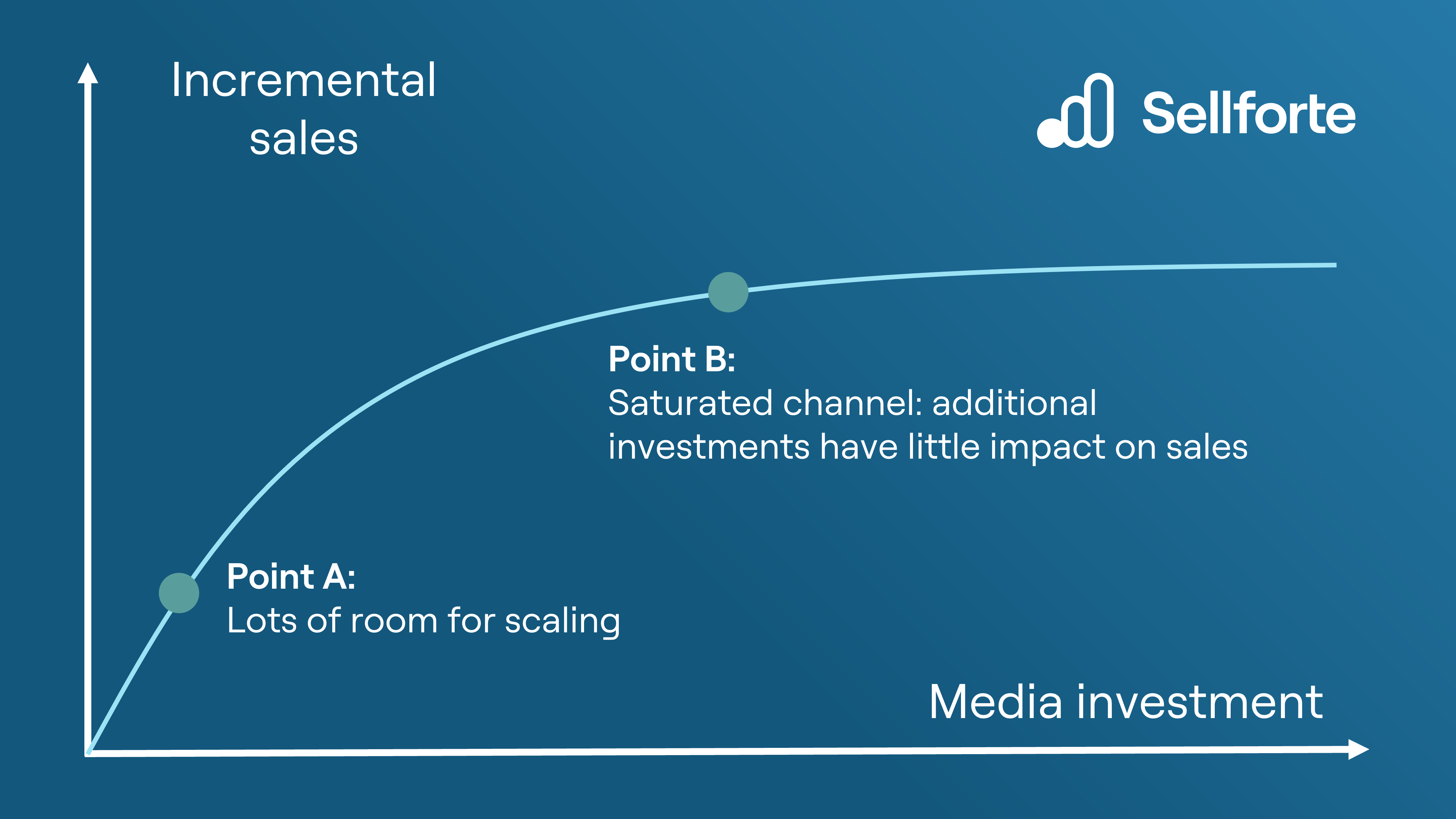
If your spend on the channel is at Point A:
✅ Increasing spend is a smart move, because the return for each new dollar is high. In other words, the marginal ROI is high.

If your spend on the channel is at Point B:
❌ Increasing spend is a bad idea: Your channel has hit a saturation point, where additional spend generates minimal extra sales. In other words, the marginal ROI is low.

Use-case 2: Evaluate Where to Invest More by Comparing Channels

In the previous example, we assessed the saturation level for an individual channel. Now let's look at another use-case: You just got more marketing budget, and need to decide which channels to invest the additional budget to.

You have two options:
1️⃣ Channel A with ROI = 5
2️⃣ Channel B with ROI = 6.

At first glance, channel B looks better, because it has higher ROI. But raw ROI isn’t the whole story. The key is to understand what is the channel that brings highest return for the next invested dollar.

Looking at the response curves and the current investment levels (circle = current spend level) in the picture below, we see that

• Additional investments to Channel A continue yielding fairly high returns.
• Additional investments to Channel B have very little incremental revenue impact.

This means that despite its higher average ROI, channel B is more saturated than channel A. As a marketer, it is smarter for you to invest the additional budget to Channel A, because it still has room for efficient growth. 

The visual logic in this example can also be turned into a mathematical concept: Marginal ROI. Marginal ROI answers the question: "If an additional euro/dollar is invested into the channel, how much additional sales will the channel drive?". It can be calculated as derivative of the response curve at a specific investment level. 

Types of Advertising Response Curves

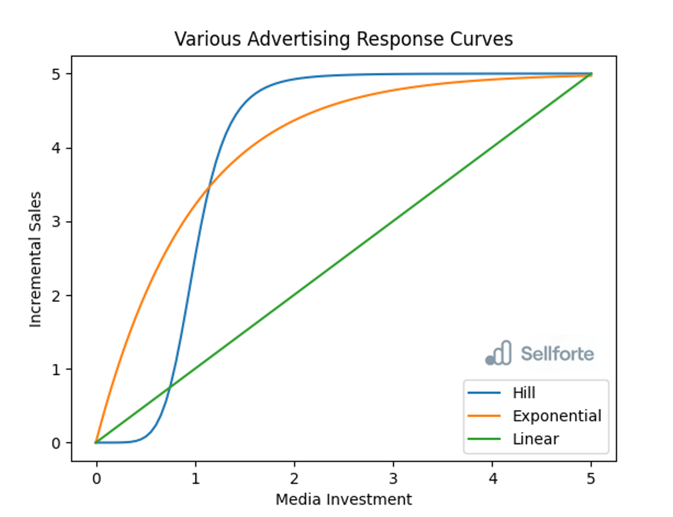
While there are several types of curves used, we'll focus on three principal ones: linear, diminishing returns, and the S-shaped or Hill curve.

Linear Response Curve

This is the simplest form of response curve and assumes a direct, proportional relationship between ad spend and consumer response. Every incremental dollar spent on advertising yields a consistent increase in response. While this model is straightforward and easy to understand, it rarely occurs in the real world because it doesn't account for saturation or diminishing returns. This is because if all channels have linear curves, that means that one channel is always better than others and we should always allocate money there. Therefore, since the linear curve has no saturation point, that means that if we more than 1 euro of incremental sales per 1 euro spend, then we can make infinite money.

Exponential or Diminishing Returns Curve

This curve is a concave function that acknowledges that not every advertising dollar will yield the same level of return. At the initial stages, each additional dollar spent on advertising results in a significant increase in response. However, as ad spend increases, the incremental benefit starts to decrease, leading to diminishing returns. This curve is more realistic than the linear curve, but it still doesn't consider the potential initial acceleration of returns when ad spend is very low. Essentially, the first euro/dollar you invest in media spend has the highest ROI, all the other ones that follow have a slightly lower impact until they reach a plateau. Read more about diminishing return curves in our blog post and in the Support Center article here.

S-shaped or Hill Curve

This curve, often modeled by a Hill function function, captures both the initial period of increasing returns and the eventual stage of diminishing returns. The curve is initially steep, indicating a substantial return on minimal ad spend. As the spend increases, the curve begins to flatten, reflecting diminishing returns. This curve is seen as the most accurate as it takes into account the entire journey of the ad spend impact, from low spends to market saturation. For some parameters, the Hill Curve, can look like an ‘Exponential curve’ where we have diminishing returns right from the start. Therefore, this is a very flexible model because it can determine whether the Hill Curve for some channels should have a more pronounced S shape or look rather Exponential.

What are the differences between the Advertising Response Curves?

The most probable answers are: feasibility and accuracy.

While the S-shaped or Hill curve is widely regarded as the most comprehensive function for Response Curves, they are relatively rare in empirical data. This rarity is largely due to the inherent characteristics of real-world advertising data. The formation of an S-shaped curve requires considerable variance in advertising spend data as It needs to capture both the initial phase where increases in ad spend lead to substantial returns (the rising section of the 'S'), and the phase where further ad spend yields diminishing returns (the plateauing section of the 'S'). To fully form an S-shaped curve, it would require data from ad spends that are low enough to be in the increasing returns section and high enough to be in the diminishing returns section.

Essentially, it rarely happens that a retailers possesses the necessary amount of data to construct an accurate S-shaped curve. In practice, many businesses do not have such a broad range in their advertising budget for a single campaign, limiting the potential for substantial variance. Campaigns tend to be optimized towards a certain level of spend based on past experiences, budget constraints, or target audience size, which often does not allow for the broad range of spend needed to empirically observe an S-curve.

A linear response curve, which implies a constant incremental increase in consumer response (like sales) for every additional dollar spent on advertising, is largely a theoretical construct. In reality, this model rarely holds true due to various factors that influence consumer response. Therefore, this curve is also a limited representation of the ARC since in reality all marketing efforts have a saturation point. After a certain level of advertising, nearly all potential customers have been reached, and any further advertising won't significantly increase consumer response. Consumers can become less responsive or even averse to repeated exposure to the same advertising, reducing the effectiveness of additional ad spend. Therefore, using a linear response curve as a representation for the performance of marketing efforts is not just hopeful but also damaging at a certain point. Moreover, please remember our previous argument on infinite money.

Exponential or diminishing return curves are the most realistic functions for representing Response Curves in most real-world scenarios. The function begins with the premise that each additional dollar spent on advertising initially results in a significant increase in the desired response—be it sales, conversions, or brand awareness. This is primarily due to the low base of advertising spend, where every new exposure can tap into a new segment of the target audience.

However, as the advertising budget continues to increase, the incremental gains start to taper off. The rationale behind this diminishing effect includes factors such as audience saturation (where nearly all potential customers have already been reached) and advertising fatigue (where consumers become less responsive as they're repeatedly exposed to the same advertisement).

Choosing the appropriate type of Advertising Response Curve is crucial for several reasons:

1. Realistic Expectations: Selecting the correct curve can provide a more accurate prediction of the advertising campaign's outcomes. This allows for more realistic goal-setting and better alignment of expectations across the team.
2. Budget Optimization: Understanding the nature of returns on ad spend helps in optimizing the advertising budget. The right curve can indicate the level of spend that maximizes returns without wastage.
3. Strategy Adjustment: The appropriate curve can signal when it may be necessary to adjust the advertising strategy, such as when diminishing returns or market saturation points are reached.
4. Performance Measurement: Choosing the correct curve contributes to a more accurate evaluation of advertising performance, supporting informed decision-making for future campaigns.
5. Improved ROI: Ultimately, the correct Advertising Response Curve helps improve the Return on Investment (ROI) by guiding strategic decisions and facilitating more effective and efficient use of advertising resources.

How to build an Advertising Response Curve?

In the advertising industry, it is the industry standard to model Response Curves using mathematical functions. Building an Advertising Response Curve is a data-driven process that is typically conducted during the running of Marketing Mix Modeling (MMM). MMM is a statistical analysis technique used to estimate the impact of various marketing tactics on sales and predict the impact of future sets of tactics. Open-source MMM libraries such as PyMCMarketing or Meridian often utilize these standard curves. Hill function is used for S-shape curves. PyMCMarketing uses logistic curve (which behaves a bit like our negative exponential - it’s diminishing return), and then Meridian uses Hill function. You can use a self serve solution such as the previously mentioned libraries or you could choose a SaaS provider to build and host the model for you. However, the baseline is that you need an MMM to successfully build an Advertising Response Curve for your marketing strategy.

Here is a general process to build an Advertising Response Curve:

1. Identify Your Assumptions: Before running the MMM, decide on the expected shape of your Response Curve based on historical data and market knowledge. You might assume a diminishing returns curve, for instance, which is common in many marketing scenarios. The choice of the curve will have a broader impact on your MMM, including the computing time needed to calculate the curve.
2. Run the MMM: Input your advertising data into the MMM. This will usually include data on different marketing tactics, such as digital, print, television advertising, and so forth, along with corresponding sales data. The data should span a considerable period to capture variability in ad spend and response. Depending on the size of your business, you might want to consider at least two years of data.
3. Estimate Curve Parameters: When running the MMM, it's not just about estimating the impact of each marketing channel. The model also estimates the parameters for the assumed Response Curve shape. This is done through a process of iterative optimization, where the model attempts to fit the parameters so that the Response Curve best matches the observed data.
4. Incorporate Priors: The model uses not only the data at hand but also "priors", which are assumptions or knowledge about the expected values or range of the parameters. These priors can be based on industry standards, previous studies, expert opinions, or business intuition. They help to guide the parameter estimation, particularly when data is sparse or noisy.
5. Validate and Refine: Once the model has estimated the Response Curve parameters, validate the curve against real-world outcomes. If the Response Curve does not accurately represent the observed data, you may need to refine your initial assumptions about the curve shape or adjust the priors.

Advertising Response Curves Transformations

During the validation process, there are two common transformations applied in MMM: the carryover (or adstock) transformation and the response curve transformation. These are mathematical adjustments made to the data to better capture the real-world effects of marketing activities.

Carryover (Adstock) Transformation: This transformation takes into account the lagged or delayed effects of marketing activities. It's based on the premise that the impact of advertising on consumer behavior doesn't end immediately when the campaign ends but continues over a period of time. This 'carryover' effect is often described using an 'adstock' model. The adstock transformation allows for the decaying effect of marketing activities, recognizing that recent activities typically have a more substantial impact than older ones. By applying this transformation, the MMM can measure the mid-term impacts of advertising on sales in a more accurate manner. Read more about the Adsock/Carryover effect.

Response Curve Transformation: This transformation acknowledges the non-linear relationship between marketing spend and sales, as represented by the Advertising Response Curve. As discussed earlier, this relationship often follows a diminishing returns pattern, where the incremental benefit of additional ad spend decreases as the total spend increases. Through this transformation, the MMM can capture this non-linear relationship, and thus, it can improve the accuracy of the model's estimations and predictions.

Key takeaways

Ultimately, Response Curves are a vital tool in marketing, helping businesses understand the relationship between advertising spend and incremental sales driven by marketing. This understanding is crucial in formulating and adjusting marketing strategies, optimizing budgets, and maximizing ROI.

Here are some key takeaways from out blog post:

• Response Curve Models: While several functions exist, including linear, diminishing returns, and S-shaped or Hill curves, the diminishing returns function tends to be the most accurate in real-world scenarios. This is due to its reflection of market saturation and advertising fatigue, which lead to diminishing returns on increased ad spend.
• Importance of Response Curves: Understanding and analyzing Response Curves allow businesses to optimize advertising budgets, identify diminishing returns, inform strategic decisions, make timely campaign adjustments, and improve the overall ROI.
• Building Response Curves: This is typically done through Marketing Mix Modeling (MMM), which involves inputting advertising data, estimating curve parameters, incorporating priors, and validating and refining the model. Transformations, specifically carryover (adstock) and response curve transformations, are crucial in capturing the delayed effects and non-linear response of advertising.

Curious to learn more? Start a Free Trial with Sellforte

Lauri Potka, Chief Operating Officer

Lauri Potka is the Chief Operating Officer at Sellforte, with over 15 years of experience in Marketing Mix Modeling, marketing measurement, and media spend optimization. Before joining Sellforte, he worked as a management consultant at the Boston Consulting Group, advising some of the world’s largest advertisers on data-driven marketing optimization. Follow Lauri in LinkedIn , where he is one of the leading voices in MMM and marketing measurement.