Advertising response curve – The curves that make-or-break campaign profitability

As in mountain climbing, you need to know when you’re closing in on the summit to avoid overdoing your next move.

So, you’ve successfully attributed the sales and profit uplifts for your latest marketing campaign. It seems that the media channels X, Y and Z did exceptionally well, whereas A, B & C failed to deliver on the sales budget. So, you double down on X-Y-Z and pull investments from the ABC, right?

Even though tempting, none of us are going to do that, because we know effectiveness rarely scales. And knowing where you stand on that effectiveness scale is one of the most important insights to gain through Marketing Mix Modeling.

Why is advertising response curve so important, then?

Because you want to get on top of that ROMI mountain, and the advertising response curve acts as an altimeter on that journey.

What is an Advertising Response Curve?

In a nutshell response curves reveal the elasticity of your media investments, so how much more sales/profit 1€ of incremental media investments would generate. This depends on the point you’re looking at the elasticity. To oversimplify things, the more you invest in one media channel, the smaller the marginal benefit you’ll get out of each invested euro or dollar.

Discovering your advertising response curves through rigorous data analysis has a profound impact on how marketing is perceived in the company by enabling three key features:

Identify saturation points

As mentioned in the beginning, it’s important not to overdo your next move after successful climb or campaign. You want to find the steepest mountain, but you don’t want to fly off the edge by not stopping at the summit point, or saturation point as it’s called in marketing.

If you have previous experimentations or enough data to extrapolate what if-scenarios, you should have an understanding how incremental spend would drive sales and profit.

Again, to oversimplify “a bit”, you should have 1,1 ROI for the incremental investment to justify this action. But as we’ll learn below, profitability can be relative when it comes to ROIs.

Optimize Media-Mix

In addition to understanding how steep ridge you’re going up, you also want to know what kind of ridges you could be ascending. For example, the previously-lucrative 1,1 ROI becomes extremely undesirable investment if you know the incremental ROI in some other media channel is between 2 and 3. Which is also poor choice, when channel O (omicron) enters the mix and shakes things up.

Which brings us to the art of optimizing (marketing investments). It is easy to generate more sales by driving up the media investments, or fabricating remarkable ROI metrics by dropping the investments to a low level. But discovering the most effective media channels in respect to the whole media mix is not a small feat.

And that’s even before we talk about the correlation between the channels. But that’s a topic for some other blog post.

Effective marketing investment management requires understanding which engines you could and should rev up, and which to cool down.

Triangulate Measurement

Finally, advertising response curves introduce more credibility to the numbers through triangulation. This is especially important during financial planning, where you need to convince top management that the changes you’re recommending will lead to the forecasted results.

There are three major shapes for advertising response curves: Linear, concave & S-curve shapes.

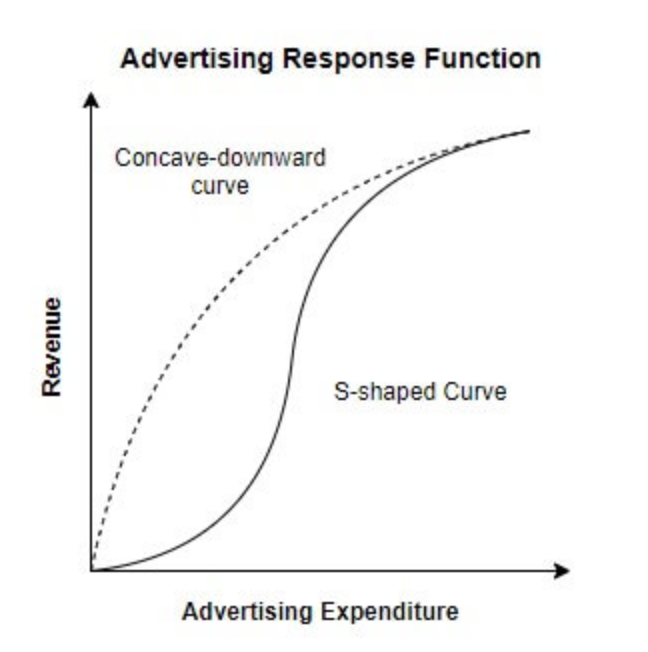
Linear response curve is the rarest shape of the response curves, and it captures events in which advertising has a direct impact on sales in a linear fashion. This is often a result of linear regression combined with insufficient data and/or previously low investment levels (which don’t give any indication about the saturation point).

Concave response shapes represent more common scenario. In this scenario advertising has a strong impact on sales in the beginning (reaching new audiences via new media channels), but this impact starts to diminish quickly after certain point, and finally saturates completely. A good example of this could be for example phones: No matter how much you advertise, after certain point consumers won’t buy additional phones no matter what.

The third major shape is the S-curve, which is arguably the most common one in real-life marketing scenarios. You see, advertising is a funny thing as it usually requires scale and frequency to work. It seems that ads cause consumption with a direct impact, but in reality we’ve been “softened” by multiple exposures earlier, and eventually give in to the temptation.

This is why media agencies usually recommend minimum spend levels for specific media channels, like TV.

S-curves are, however, somewhat rare to come across empirically. This is due to the fact that ending up with a S-curve requires substantially more variance in the data than what the usual datasets include.

How to build an Advertising Response Curve?

Now that we’ve established the context of advertising response curves, it’s time to review which factors affect what the curve eventually looks like (and what you need to consider when measuring your next response curve).

There are four effects that shape the response curves: Current Effect, Carryover Effect, Competitive Effect and Dynamic Effects.

Current Effect

This is the incremental revenue that can be attributed to an ad on the same time period this commercial is being aired. As there’s usually more than one active ad within the time frame, time series analysis is recommended to isolate each channel’s sales impact.

Current effects shape the advertising response curve through diminishing returns phenomenon (or in the rare cases, the absence of it). If the sales uplift for incremental investments remains more or less constant, we’re looking at linear curve. But if the returns diminish exponentially, as they normally do, the advertising response curve is concave.

Carryover Effect

As mentioned above, consumers are not as linear decision makers as some models would like to assume. Especially brand campaigns tend to affect the decision-making processing after the campaign has come to an end.

Most ads affect the buying behavior also after the campaign has ended. Attributing the carryover effect is not, however, as easy as one would think. But it is possible to measure with hard numbers. Cartoon by marketoonist.com

Carryover Effect can be estimated through time series analysis as well, but it also requires information about your Base Sales, as you need to know the post-campaign incremental sales. Another method is ad-stocking that utilizes decay rates to attribute post-campaign sales.

In case there’s lagged impact or carryover effect, the saturation point moves further down the graph.

Competitive Effect

Normally every marketer faces competition when it comes to marketing. Competitors’ advertising can be complementary (e.g. when introducing new products to the market), but usually this leads to a negative impact on your advertising effectiveness.

Competition is one of the reasons for S-shaped curves, as it takes certain level of scale and frequency to push through the sea of noise.

Dynamic Effects

Dynamic effects refer to changes in sales that are caused by other than the above-mentioned effects, when the advertising intensity remains the same. Most common ones are weather and seasonality, but based on the industry and market additional variables such as macroeconomic factors can generate dynamic effects.

Dynamic effects make the advertising response curves, well, dynamic, as they can dramatically change how incremental investments drive sales. A good example of this would be sporting goods retail sector, which winter sales are largely depended on the weather. A proper winter can twist the curve to an almost convex shape, whereas the opposite will almost surely lead to concave (and very flat) response curve.

Conclusion

Advertising response curves are an excellent tool in combining different scenarios and optimizing the media spend distribution. They can help you to understand how much headroom is left with each media channel and avoid over- or underinvesting in your next marketing campaign.

The biggest challenge is, however, that in most cases the response curves are more or less correlated with each other. Changing the investment level in one channel can affect other channels’ performance as well, so finding the perfect balance requires world-class modeling tools as well as rigorous testing and learning approach.

Moreover, one should consider moving to continuous modeling, as the response curves are not constant, but change over time.

Curious to learn more? Book a demo.